Martingale posteriors in modern AI

Trial Lecture, University of Oslo

Simen Eide

2025-11-28

Agenda

Target audience: master students with some knowledge about Bayesian statistics

• Motivational LLM In Context Learning
• Traditional Bayesian review
• Predictive Bayesian introduction
• Predictive resampling algorithm
• Some theory
• Applications
• Conclusion

LLM In-Context Learning

• Assume we ask an LLM to solve the following problem

Where should this person go on holiday based on some information of that person?

x: Simen just defended his PhD in Machine Learning and enjoys paragliding
y:

LLM In-Context Learning

• Assume we ask an LLM to solve the following problem

• Collect some few shot examples

Where should this person go on holiday based on some information of that person?

x: Anders is a physicist and likes to discuss philosophy
y: destination=Rome

x: Kamilla enjoys skiing and works at the local university
y: destination=Alps

x: Simen just defended his PhD in Machine Learning and enjoys paragliding
y:

LLM In-Context Learning

• Assume we ask an LLM to solve the following problem
• Collect some few shot examples
• Let the LLM generate additional examples

• Repeat and record answer

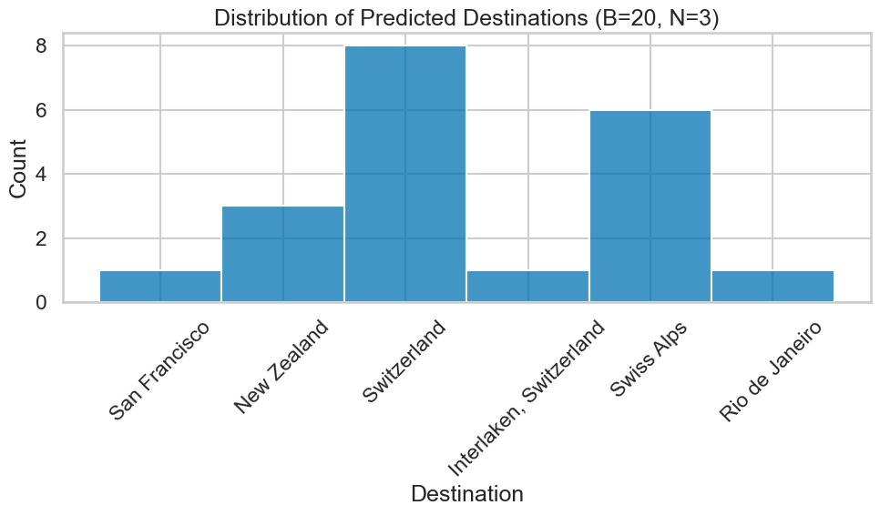
Where should this person go on holiday based on some information of that person?

x: Anders is a physicist and likes to discuss philosophy
y: destination=Rome

x: Kamilla enjoys skiing and works at the local university
y: destination=Alps

x: Maria is retired and spends her time gardening and traveling
y: destination=Madeira

x: Sven just quit his job and is now playing in a band with his friends.
y: destination=Nashville

x: Elias is in military conscription and is considering studying engineering afterward
y: destination=Berlin

x: Ingrid is a medical resident finishing her fourth year of specialty training
y: destination=The Well

x: Thomas just became a partner at a consulting firm and enjoys sailing
y: destination=Maldives

x: Simen just defended his PhD in Machine Learning and enjoys paragliding
y:

Valid? Posterior predictive?

Traditional Bayesian approach

Traditional Bayesian approach

• Collect data points from an unknown distribution \(F_0\)
• Define a prior \(\pi(\theta)\) and a likelihood \(f_\theta(y)\)
• Compute the posterior \(P(\theta | y_{1:n})\)
• Compute the posterior predictive \(P(y | y_{1:n})\)

• We have collected \(y_{1:n}\) data points from an unknown distribution \(F_0\).
• Assume \(F_0\) has a true density \(y_i \sim f_{\theta_0}\) given by a true parameter \(\theta_0\).
• Goal: Find probable values of \(\theta_0\) given the data \(y_{1:n}\).

• Prior \(\pi(\theta)\)
• Sampling density \(f_{\theta}(y)\)
• Likelihood \(f_\theta(y) = p(y_{1:n} | \theta) = \prod_{i=1}^n f_\theta(y_i)\)

Posterior

\[ P(\theta | y_{1:n}) = \frac {\pi(\theta) p(y_{1:n} | \theta )} {\int \pi(\theta) p(y_{1:n} | \theta ) d\theta} \tag{1}\]

Posterior predictive

We can compute the distribution of a new data point \(y\) given the observed data \(y_{1:n}\) by using the posterior predictive

\[ P(y | y_{1:n}) = \int f_{\theta}(y) \pi(\theta | y_{1:n}) d\theta \tag{2}\]

Prior beliefs on Neural Network parameters?!

• Neural networks are black box models
• How can we have any prior knowledge about the parameters in hidden layers?

• Neural networks are black box models
• We have no intuition here(!)

Standard answer:

We dont care, we just want to use it for variability

Today: Start at a different point

• Instead, define the predictive distribution:

\[P(y_{n+1} | y_{1:n})\]

• More natural to define the predictive distribution instead of prior+likelihood?

Predictive Bayes Motivation

Compute statistics from an infinite population

Holmes and Walker (2023)

• Think of bayesian ucertainty to originate from missing data:

The assumption behind most, if not all, statistical problems is that there is an amount of data, \(x_{comp}\), which if observed, would yield the problem solved.

For example:

• Consider i.i.d. observations from an infinite population.
• We have collected \(y_\text{obs} := y_{1:n}\)
• The missing data are then \(y_\text{mis} := y_{n+1:{\infty}}\)
• If we had access to the full data \(y_{comp} := \{y_\text{obs}, y_\text{mis} \}\), we could compute any statistics of interest with near zero uncertainty.

Simulate the missing data

• Therefore, we can find a posterior distribution, not by specifying priors and likelihoods, but by specifying the distribution of the missing data given the observed data!

Holmes and Walker (2023)

The Bayesian posterior can be written as

\[ \begin{aligned} \pi(\theta | y_\text{obs}) =& \int \pi(\theta, y_\text{mis} | y_\text{obs}) dy_\text{mis} \\ =& \int \pi(\theta | y_\text{comp}) P(y_\text{mis} | y_\text{obs}) dy_\text{mis} \end{aligned} \]

• We can make \(y_\text{comp}\) arbitrarily large
• Replace the conditional posterior with a point estimate \[\pi(\theta | y_\text{comp}) = \delta_{\hat{\theta}(y_\text{comp})}(\theta)\]
• Integrate over the missing data

Just need to define \(P(y_\text{mis} | y_\text{obs})\) …

Predictive resampling

Fong, Holmes, and Walker (2022)

Way to sample the missing data given a one step ahead predictive distribution \(P(y_{i+1} | y_{1:i})\)

\(y_{comp} = y_{1:\infty} \approx y_{1:N}\) for some large N.

\[ P(y_{n+1:N} | y_{1:n}) = \prod_{i=n}^N P(y_{i+1} | y_{1:i}) \]

Step 1: Simulate \(y_{n+1:\infty}\) by N one step ahead predictions \(P(y_{i+1} | y_{1:i})\)

Step 2: Compute the quantity of interest \(\theta(y_{1:N})\) on the full dataset

Repeat B times to get a posterior distribution of the quantity of interest

theta_samples = np.zeros(B)
for b in range(0,B):
    y = np.zeros(N)
    y[:n] = y_obs
    for i in range(n+1,N):
        y[i] = p_i(y[1:(i-1)])

    theta_samples[b] = theta(y)

NB: Need to define a valid \(P(y_{i+1} | y_{1:i})\)

Example 1 (problem)

Adapted example from Fong, Holmes, and Walker (2022)

Assume we have the model \[ P(\theta):= \pi(\theta) = N(\theta | 0,1) \\ P(y|\theta):=f_\theta(y) = N(y | \theta, 1) \]

Conjugate prior gives closed form posterior

\[ P(\theta | y_{1:n}) = N(\theta | \bar{\theta_n}, \bar{\sigma_n}^2 ) \] where \[ \bar{\theta_n} := \frac{\sum_{i=1}^n y_i}{n+1}, \bar{\sigma}_n^2 := \frac{1}{n+1} \]

and posterior predictive \[ P(y | y_{1:n}) = N(y | \bar{\theta_n}, \bar{\sigma_n^2} + 1)\]

Set the true parameter \(\theta =2.0\), and then collect \(n=50\) values:

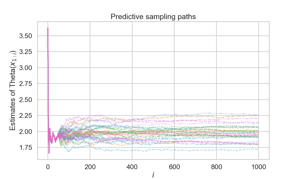
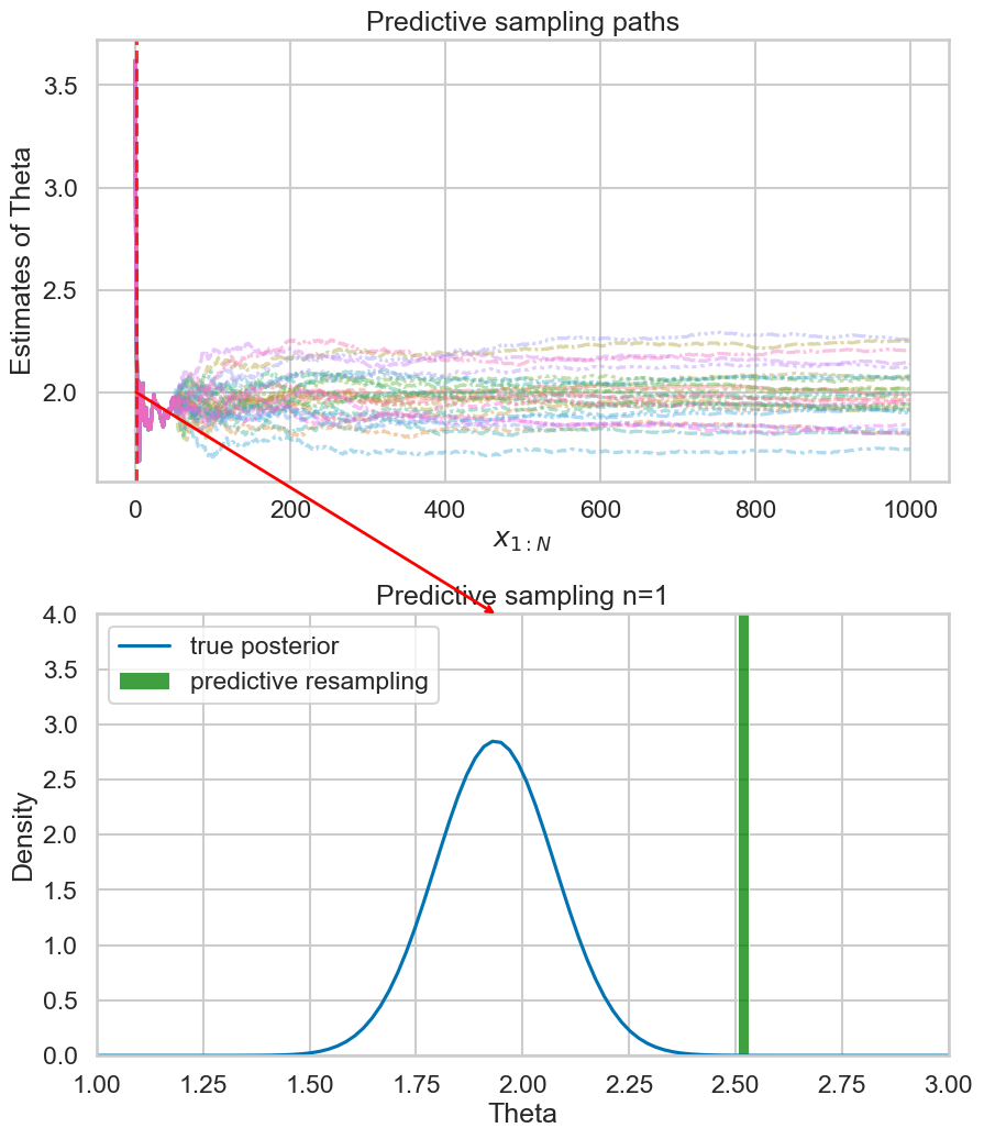
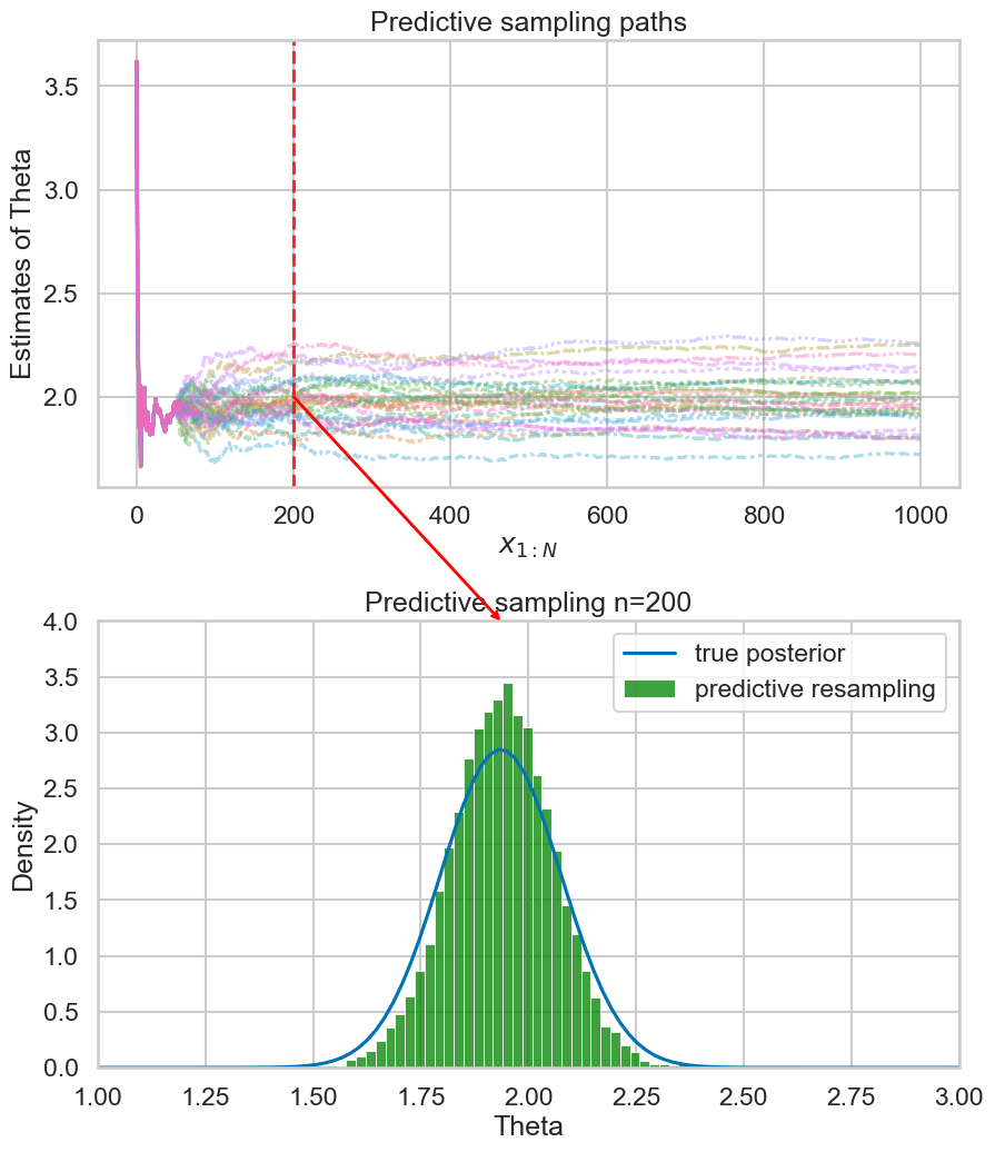
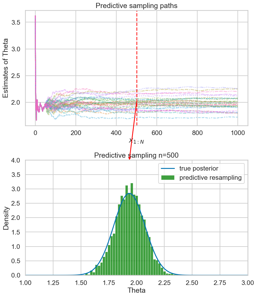
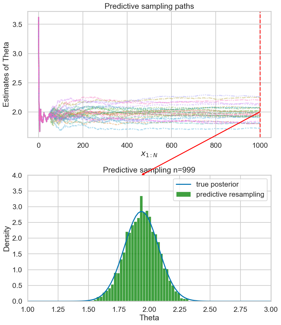
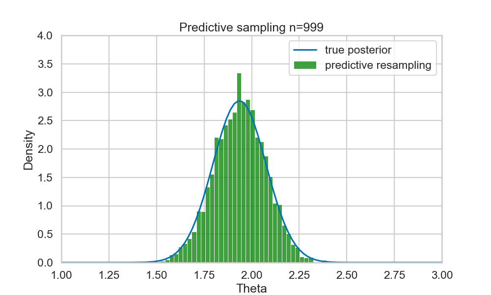
Example (run predictive resampling)

• Assume we made a good guess and think that the posterior predictive is a good function to sample from

• Let the predictive distribution be the true posterior predictive: \[ P(y_{i+1} | y_{1:i}) = N(y | \bar{\theta_i}, \bar{\sigma_i^2} + 1)\]

• Step 1: For \(i=n,...,N-1\):  Sample \(y_{i+1} | y_{1:i}\) from the posterior predictive

• Step 2: Compute the point estimate of \(\theta\) given the full data \(y_{1:N}\): \[ \hat{\theta}(y_{1:N}) = \frac{\sum_{i=1}^N y_i}{N+1} \]

• Repeat B times to get posterior samples of \(\theta\)

Why is this useful?

Recap

• We can find a posterior statistics \(\theta(y_{1:N})\) if we have a valid \(P(y_{i+1} | y_{1:i})\).
• Do not need to define prior or likelihood

Specification

• Priors on BNN parameters lack a clear interpretation
• Maybe its more intuitive to define a predictive distribution?
• \(P(y_{i+1} | y_{1:i})\) feels similar to many black box models we have today

Computation

• Predictive resampling instead of MCMC
• Predictive resampling can be parallelized
  • 10-100x speedups

Theory on the predictive distributions

What predictive distributions does this work for?

Fortini and Petrone (2025)

We now have a sequence \((Y_n)_{n\ge1}\) where we can generate new samples with the predictive distribution \(P_n := P(y_{n+1} | y_{1:n})\).

However, when does this technique give us an actual data distribution \(F_0\)?

• Have a \(P(y_{i+1} | y_{1:i})\) that will generate a sequence \((Y_i)_{i\ge n}\)

• When \((Y_i)_{i\ge n}\) give us a data distribution \(F_0\)? i.e. when does

\[ (Y_n)_{n\ge1} | F_0 \] exists.

In this section we will:

• Introduce a requirement on the sequence \((Y_i)_{i\ge1}\) that makes it possible to define a prior
• Then relax this requirement
• End up with a requirement that \(P(y_{i+1} | y_{1:i})\) is a martingale.

de Finetti’s Theorem

Definition 1 \((Y_i)_{i\ge1}\) is exchangeable if

\[ (Y_{\sigma(1)}, Y_{\sigma(2)},...) \sim (Y_1, Y_2, ..) \]

for every finite permutation \(\sigma\) of \(\mathbb{N}\) .

Theorem 1 (de Finetti’s Theorem)  

There exist \(F_0\) such that \((Y_i) | F_0\)
if and only if
\((Y_i)\) is exchangeable.

If we can construct a \(P(y_{i+1} | y_{1:i})\) so that the resulting sequence \((Y_i)_{i\ge n}\) is exchangeable, then we have our familiar traditional Bayes framework

In reality, hard to use exchangeability

Relaxing exchangeability

c.i.d. : “conditionally on the past, all future observations are identically distributed” Stationarity: A stationary sequence is a random sequence whose joint probability distribution is invariant over time

Theorem 2 (Kallenberg 1988)
“Exchangeability = Stationarity + conditionally identically distributed”

So let us remove stationarity…

Definition 2 (Conditionally identically distributed (c.i.d.)) A sequence \((Y_n)_{n\ge 1}\) is c.i.d. if it satisfies

\[ P(Y_{n+k} | y_1, ..., y_{n}) = P(Y_{n+1} | y_1, .., y_{n}) \] for all \(k\ge1\).

All future observations share the same conditional distribution given the past

Martingale

Definition 3 (Conditionally identically distributed (c.i.d.)) A sequence \((Y_n)_{n\ge 1}\) is c.i.d. if it satisfies

\[ P(Y_{n+k} | y_1, ..., y_{n}) = P(Y_{n+1} | y_1, .., y_{n}) \] for all \(k\ge1\).

All future observations share the same conditional distribution given the past

This is equivalent to saying:

Definition 4 (Martingale of the predictive distribution) \[ E[P(Y_{i+2} \in A | y_{1:{i+1}}) | y_{1:i}] = P(Y_{i+1} \in A | y_{1:i}) \] for all \(A\) and all \(i\).

Still have many desirable properties

• \((Y_i)_{i\ge n}\) converge to a distribution \(F_0\),
• \((Y_i)_{i\ge n}\) are identically distributed,

• \((Y_i)_{i\ge n}\) are asymptotically exchangeable
• The empirical distribution of \((Y_i)_{i\ge n}\) converges to \(F_0\)

Applications

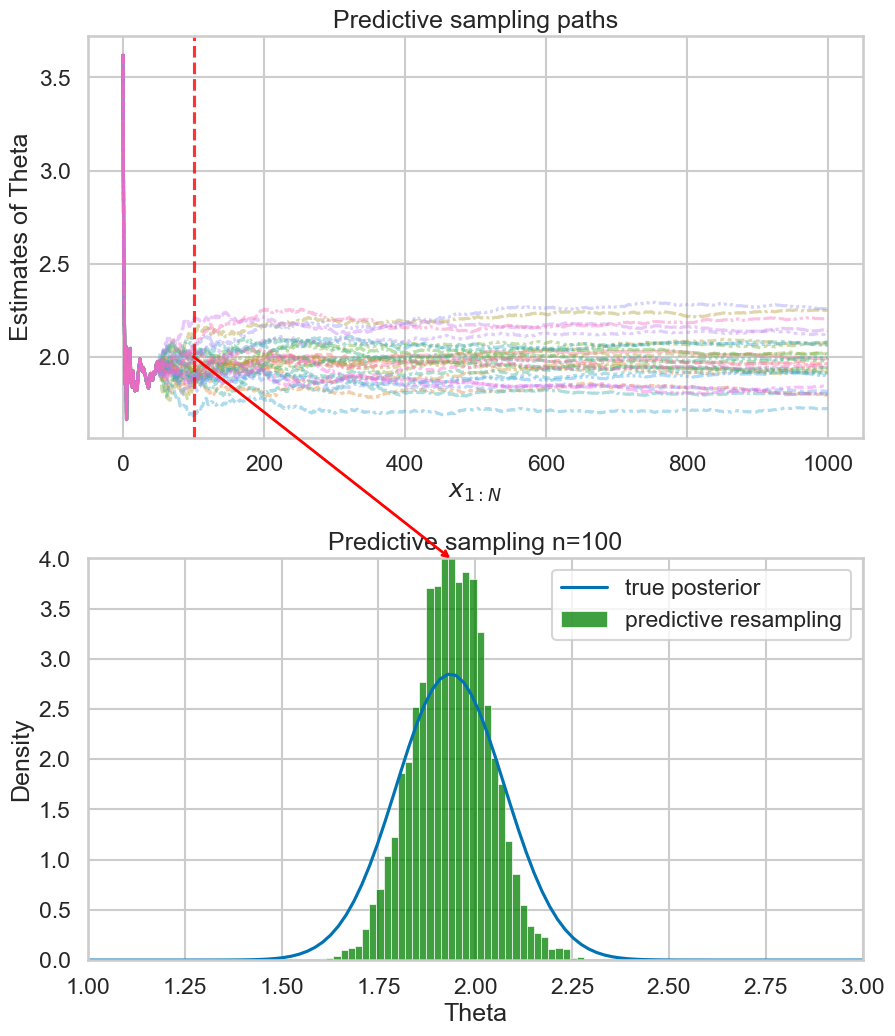
Example 1: Empirical predictive

• Remember example:
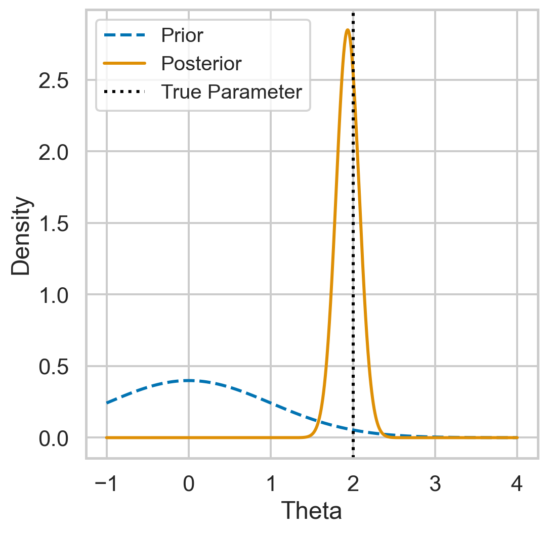
  • \(Y_i \sim N(\theta, 1)\)
  • \(\theta=2\)

• If we instead of the true posterior predictive assume an empirical predictive on the collected data \(y_{1:n}\):

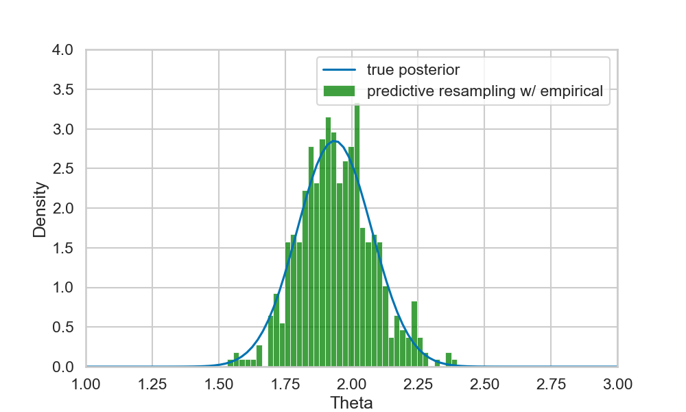
• Works but “worse model”

Are LLMs martingales?

• Check whether \(P(y_{i+1}|y_{1:i})\) is a martingale

• Note: \(y_{i+1}\) is not the next token!

Where should this person go on holiday based on some information of that person?

x: Anders is a physicist and likes to discuss philosophy
y: destination=Rome

x: Kamilla enjoys skiing and works at the local university
y: destination=Alps

x: Maria is retired and spends her time gardening and traveling
y: destination=Madeira

x: Sven just quit his job and is now playing in a band with his friends.
y: destination=Nashville

x: Elias is in military conscription and is considering studying engineering afterward
y: destination=Berlin

x: Ingrid is a medical resident finishing her fourth year of specialty training
y: destination=The Well

x: Thomas just became a partner at a consulting firm and enjoys sailing
y: destination=Maldives

x: Simen just defended his PhD in Machine Learning and enjoys paragliding
y:

Are LLMs martingales?

Falck, Wang, and Holmes (2024)

• Falck, Wang, and Holmes (2024) studies martingale property of LLMs in-context learning empirically

• Tests three LLMs:
  • gpt-3.5,
  • llama-2-7b
  • mistral-7b

• Tests three datasets:
  • Bernoulli,
  • Gaussian,
  • Synthetic natural language dataset

• Result: No.

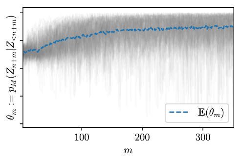
• The expected probability drifts as \(i\) increases

• Suggests tools or fine tuning to make LLMs more like martingales

Tabular Prior Fitted Networks (TabPFN)

Hollmann et al. (2023), Nagler and Rügamer (2025), Ng et al. (2025)

Why does the dirichlet mixture help?

• TabPFN: pretrained transformer on tabular data (Hollmann et al. (2023))

• Observe the same non-martingale property in TabPFN (Nagler and Rügamer (2025))

Two different approaches:

Nagler and Rügamer (2025)

Only use tabPFN on the first step \(P(y_{n+1} | x_{n+1}, z_{1:n})\), then a Dirichlet process mixture for the rest.

Ng et al. (2025)

“Ignores” theoretical requirements, checks convergence empirically and says its “good enough”.

Conclusion

Conclusion

• Introduced a new, alternative Bayesian framework
• Specify predictive distributions instead of priors and likelihoods
• Hints at being able to insert our favourite black-box auto-regressive model
• Highly parallizeable
• Limitation: Difficult/unsure how to specify valid predictive distributions

Future (/current) work

• Show that different models (predictive distributions) are martingales
• Relaxation of the martingale posterior (e.g. Battiston and Cappello (2025))
• Empirical robustness (e.g. Ng et al. (2025))

Half baked (LLM)-ideas

• “LLMs are not row-invariant due to positional embeddings” Ng et al. (2025)

• Can we design new, “local” positional embeddings architectures are row-invariant?

• Update parametric models inside predictive resampling. LLM posteriors?

:::

References

Battiston, Marco, and Lorenzo Cappello. 2025. “Bayesian Predictive Inference Beyond Martingales.” arXiv. https://doi.org/10.48550/arXiv.2507.21874.

Falck, Fabian, Ziyu Wang, and Chris Holmes. 2024. “Are Large Language Models Bayesian? A Martingale Perspective on in-Context Learning.”

Fong, Edwin, Chris Holmes, and Stephen G Walker. 2022. “Martingale Posterior Distributions.” Journal of the Royal Statistical Society Series B: Statistical Methodology 85 (5): 1357–91. https://doi.org/10.1093/jrsssb/qkad005.

Fortini, Sandra, and Sonia Petrone. 2025. “Exchangeability, Prediction and Predictive Modeling in Bayesian Statistics.” Statistical Science 40 (1): 40–67. https://doi.org/10.1214/24-STS965.

Hollmann, Noah, Samuel Müller, Katharina Eggensperger, and Frank Hutter. 2023. “TabPFN: A Transformer That Solves Small Tabular Classification Problems in a Second.” arXiv. https://arxiv.org/abs/2207.01848.

Holmes, Chris C., and Stephen G. Walker. 2023. “Statistical Inference with Exchangeability and Martingales.” Philosophical Transactions of the Royal Society A: Mathematical, Physical and Engineering Sciences 381 (2247): 20220143. https://doi.org/10.1098/rsta.2022.0143.

Nagler, Thomas, and David Rügamer. 2025. “Uncertainty Quantification for Prior-Data Fitted Networks Using Martingale Posteriors.” arXiv. https://doi.org/10.48550/arXiv.2505.11325.

Ng, Kenyon, Edwin Fong, David T. Frazier, Jeremias Knoblauch, and Susan Wei. 2025. “TabMGP: Martingale Posterior with TabPFN.” arXiv. https://doi.org/10.48550/arXiv.2510.25154.

BONUS

Parametric models

Holmes and Walker (2023)

• Consider a data model \(f(y | \theta_0)\)
• Let \(\hat{\theta}_n = \theta(y_{1:n})\) be an unbiased MLE estimate of \(\theta_0\) based on \(y_{1:n}\)
• Then we can sample a new point and estimate a new parameter

\[ y_{n+1} \sim f(y | \hat{\theta}_n) \\ \hat{\theta}_{n+1} = \theta(y_{1:n+1}) \]

• Idea: If uncertainty in mle estimate decreases with more data, then we can iteratively update

• \[ \theta_{m+1} = \theta_m + \epsilon_m \frac{\partial log f(x_{m+1}|\theta_m)}{\partial \theta_m} \] where \(\epsilon_m\) functions as our learning rate scheduler.

• “Gradient descent style” updates

• Gives us the “frequentist posterior”